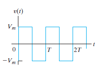
Electronic oscillators, which are extremely useful in laboratory testing of equipment, are specifically designed to create non-sinusoidal periodic waveforms. Moreover, non-sinusoidal periodic functions are important in analyzing non-electrical systems. Problems that involve fluid flow, mechanical vibration, and heat flow all make use of different periodic functions. This article will detail a brief overview of a Fourier series, calculating the trigonometric form of the Fourier coefficients for a given waveform, and simplification of the waveform when provided with more than one type of symmetry. Any periodic signal can be represented as a sum of sinusoids where the frequencies of the sinusoids in the sum are composed of the frequency of the periodic signal and integer multiples of that frequency. Using a periodic signal like a square wave to test the quality factor of a bandpass or band reject filter. In order to do this, a square wave whose frequency is the same as the center frequency of a bandpass filter is chosen. Fourier Series Overview An analysis of heat flow in a metal rod led the French mathematician Jean Baptiste Joseph Fourier to the trigonometric series representation of a periodic function. This representation of a periodic function is the starting point for finding the steady-state response to periodic excitations of electric circuits. What was discovered was that a periodic function can be represented by an infinite sum of sine or cosine functions that are related harmonically. The period of any trigonometric term in the infinite series is an integral multiple, or harmonic, of the period T of the periodic function. To visualize an understanding, below are a few waveforms produced by function generators used in laboratory testing. The Fourier series shows that f(t) can be described as f ( t ) = a v + ∑ n = 1 ∞ a n cos ( n ω 0 t ) + b n sin ( n ω 0 t ) f ( t ) = a v + ∑ n = 1 ∞ a n cos ( n ω 0 t ) + b n sin ( n ω 0 t ) (1.1) Fourier series representation of a periodic function Where n is the integer sequence 1,2,3,… In Eq. 1.1, a v a v , a n a n , and b n b n are known as the Fourier coefficients and can be found from f(t) . The term ω 0 ω 0 (or 2 π T 2 π T ) represents the fundamental frequency of the periodic function f(t) . The integral multiples of ω 0 ω 0 , i.e. 2 ω 0 , 3 ω 0 , 4 ω 0 2 ω 0 , 3 ω 0 , 4 ω 0 and so on, are known as the harmonic frequencies of f(t) . Thus n ω 0 n ω 0 is the n th harmonic term of f(t) . Before discussing Fourier coefficients, the conditions in a Fourier series need to be explained. For a periodic function f(t) to be a convergent Fourier series, the following conditions need to be met: f(t) be single-valued, f(t) have a finite number of discontinuities in the periodic interval, f(t) have a finite number of maxima and minima in the periodic interval, the integral ∫ t 0 + T t 0 ∣ f ( t ) ∣ d t ∫ t 0 t 0 + T ∣ f ( t ) ∣ d t exists, These 4 conditions are known as Dirichlet’s conditions, and are sufficient condition, not necessary conditions. Thus if f(t) meets these requirements, it can be expressed as a Fourier series. Nonetheless, if f(t) does not meet these requirements, it still can be expressed as a Fourier series; the necessary conditions on f(t) are not known. The Fourier Coefficients Having defined a periodic function over its period, the following Fourier coefficients are determined from the relationships: a v = 1 T ∫ t 0 + T t 0 f ( t ) d t , a v = 1 T ∫ t 0 t 0 + T f ( t ) d t , (1.2) a k = 2 T ∫ t 0 + T t 0 f ( t ) cos ( k ω 0 t ) d t , a k = 2 T ∫ t 0 t 0 + T f ( t ) cos ( k ω 0 t ) d t , (1.3) b k = 2 T ∫ t 0 + T t 0 f ( t ) sin ( k ω 0 t ) d t , b k = 2 T ∫ t 0 t 0 + T f ( t ) sin ( k ω 0 t ) d t , (1.4) In Eqs. 1.3 and 1.4, the subscript k indicated the k th coefficient in an integer sequence 1,2,3,…Noting that a v a v is the average value of f(t) , a k a k is twice the average value of f ( t ) cos ( k ω 0 t ) f ( t ) cos ( k ω 0 t ) , and b k b k is twice the average value of f ( t ) sin ( k ω 0 t ) f ( t ) sin ( k ω 0 t ) . To gain a better understanding of how Eqs 1.2-1.4 came from Eq 1.1, simple derivations can be used through integral relationships which hold true when m and n are integers: ∫ t 0 + T t 0 sin ( m ω 0 t ) d t = 0 ∫ t 0 t 0 + T sin ( m ω 0 t ) d t = 0 for all m, (1.6) ∫ t 0 + T t 0 cos ( m ω 0 t ) d t = 0 ∫ t 0 t 0 + T cos ( m ω 0 t ) d t = 0 for all m, (1.7) ∫ t 0 + T t 0 cos ( m ω 0 t ) sin ( n ω 0 t ) d t = 0 ∫ t 0 t 0 + T cos ( m ω 0 t ) sin ( n ω 0 t ) d t = 0 for all m and n , (1.8) ∫ t 0 + T t 0 sin ( m ω 0 t ) sin ( n ω 0 t ) d t = 0 ∫ t 0 t 0 + T sin ( m ω 0 t ) sin ( n ω 0 t ) d t = 0 for all m ≠ n m ≠ n = T 2 , = T 2 , for all m = n (1.9) ∫ t 0 + T t 0 cos ( m ω 0 t ) cos ( n ω 0 t ) d t = 0 ∫ t 0 t 0 + T cos ( m ω 0 t ) cos ( n ω 0 t ) d t = 0 for all m ≠ n m ≠ n = T 2 , = T 2 , for all m = n (1.10) In order to derive Eq 1.3, both sides of Eq 1.2 need to be integrated over one period: ∫ t 0 + T t 0 f ( t ) d t = ∫ t 0 + T t 0 ( a v + ∑ n = 1 ∞ a n cos ( n ω 0 t ) + b n sin ( n ω 0 t ) ) d t ∫ t 0 t 0 + T f ( t ) d t = ∫ t 0 t 0 + T ( a v + ∑ n = 1 ∞ a n cos ( n ω 0 t ) + b n sin ( n ω 0 t ) ) d t ∫ t 0 + T t 0 a v d t + ∑ n = 1 ∞ ( a n cos ( n ω 0 t ) + b n sin ( a n cos ( n ω 0 t ) ) d t ∫ t 0 t 0 + T a v d t + ∑ n = 1 ∞ ( a n cos ( n ω 0 t ) + b n sin ( a n cos ( n ω 0 t ) ) d t = a v T + 0 = a v T + 0 (1.11) To derive the expression for the k th value of a n a n , Eq 1.2 need to be multiplied by cos ( k ω 0 t ) cos ( k ω 0 t ) and then both sides need to be integrated over one period of f(t) : ∫ t 0 + T t 0 f ( t ) cos ( k ω 0 t ) d t = ∫ t 0 + T t 0 a v cos ( k ω 0 t ) d t ∫ t 0 t 0 + T f ( t ) cos ( k ω 0 t ) d t = ∫ t 0 t 0 + T a v cos ( k ω 0 t ) d t + ∑ ∞ n = 1 ∫ t 0 + T t 0 ( a n cos ( n ω 0 t ) c o s ( k ω 0 t ) + b n sin ( n ω 0 t ) sin ( k ω 0 t ) ) d t + ∑ ∞ n = 1 ∫ t 0 t 0 + T ( a n cos ( n ω 0 t ) c o s ( k ω 0 t ) + b n sin ( n ω 0 t ) sin ( k ω 0 t ) ) d t = 0 + a k ( T 2 ) + 0 = 0 + a k ( T 2 ) + 0 (1.12) Lastly, the expression for the k th value of b n b n by multiplying both sides of Eq. 1.2 by sin ( k ω 0 t ) sin ( k ω 0 t ) and then integrating each side over one period of f(t) . The following example explains how to use Eqs. 1.3 – 1.5 to calculate the Fourier coefficients for a specific periodic function. Finding the Fourier series of a Triangular Waveform with No Symmetry: In this example, you are asked to find the Fourier series for the given periodic voltage shown below When using Eqs. 1.3 – 1.5 to solve for a v a v , a k a k , and b k b k , the value of t 0 t 0 can be chosen to be any value. For this specific periodic voltage, the best value is zero. If a value other than that of zero, integration would become difficult. The expression for v(t) between 0 and T is: v t = ( V m T ) t v t = ( V m T ) t The equation for a v a v is: a v = 1 T ∫ T 0 ( V m T ) t d t = 1 2 V m a v = 1 T ∫ 0 T ( V m T ) t d t = 1 2 V m The value found above is the average value of the waveform shown above. The equation for the kth value of a n a n is: a k = 2 T ∫ T 0 ( V m T ) t cos ( k ω 0 t ) d t a k = 2 T ∫ 0 T ( V m T ) t cos ( k ω 0 t ) d t = 2 V m T 2 ( 1 k 2 w 2 0 cos ( k ω 0 t ) + t k ω 0 sin ( k ω 0 t ) ) = 2 V m T 2 ( 1 k 2 w 0 2 cos ( k ω 0 t ) + t k ω 0 sin ( k ω 0 t ) ) Evaluated from 0 to T. = 2 V m T 2 [ 1 k 2 ω 2 0 ( cos ( 2 π k − 1 ) ] = 0 = 2 V m T 2 [ 1 k 2 ω 0 2 ( cos ( 2 π k − 1 ) ] = 0 for all k The equation for the kth value of b n b n is: b k = 2 T ∫ T 0 ( V m T ) t sin ( k ω 0 t ) d t b k = 2 T ∫ 0 T ( V m T ) t sin ( k ω 0 t ) d t = 2 V m T 2 ( 1 k 2 ω 2 sin ( k ω 0 t ) − t k ω 0 cos ( k ω 0 t ) ) = 2 V m T 2 ( 1 k 2 ω 2 sin ( k ω 0 t ) − t k ω 0 cos ( k ω 0 t ) ) Evaluated from 0 to T. = 2 V m T 2 ( 0 − T k ω 0 cos ( 2 π k ) ) = 2 V m T 2 ( 0 − T k ω 0 cos ( 2 π k ) ) = − V m π k = − V m π k Finally, the Fourier series for v(t) is: v ( t ) = V m 2 − V m π ∑ n = 1 ∞ 1 n sin ( n ω 0 t ) v ( t ) = V m 2 − V m π ∑ n = 1 ∞ 1 n sin ( n ω 0 t ) v ( t ) = V m 2 − V m π sin ( ω 0 t ) − V m 2 π sin ( 2 ω 0 t − V m 3 π sin ( 3 ω 0 t ) − . . . v ( t ) = V m 2 − V m π sin ( ω 0 t ) − V m 2 π sin ( 2 ω 0 t − V m 3 π sin ( 3 ω 0 t ) − . . . Coming Up At this point, you should have an understanding of what a Fourier series is, what the Fourier coefficients are, and the calculations to find the trigonometric form of the Fourier coefficients for a periodic waveform. Future articles will detail average power with periodic functions as well as analyzing a circuit’s response to a waveform using the Fourier coefficients talked about in this article. Another topic that will be covered is the four types of symmetry that can be used to simplify the evaluation of the Fourier coefficients as well as the effect of symmetry on the Fourier coefficients.
[via LEKULE]
Follow us @automobileheat – lists / @sectorheat